Research - (2023) Volume 11, Issue 4
Simulation and Analysis of Imus Transport Plaza Terminal: Ridership
Gil Christian C. Alvarez, Kenneth A. Brondial, Mark Allen M. Cabutaje and Jean Allyson S. Junsay*Received: Apr 20, 2023, Manuscript No. ijcsma-23-96620; Editor assigned: Apr 22, 2023, Pre QC No. ijcsma-23-96620 (PQ); Reviewed: Apr 30, 2023, QC No. ijcsma-23-96620 (Q); Revised: May 06, 2023, Manuscript No. ijcsma-23-96620 (R); Published: May 11, 2023, DOI: 10.5281/zenodo.8086553
Abstract
Public transportation has been an essential part of everyday travel for Filipinos, Commuters or non-commuters, as it provides an option for everyone in means of making sure that people will arrive and will reach their desired place on time. Public transportation varies from jeepneys, tricycles, pedicab, multicab, buses, trains, etc. It has its advantages and disadvantages, but it helps commuters to travel from one place to another with cheaper cost and its daily availability for the public or its convenience. This project aims to model and simulate how and what is the process of passenger flow and the vehicle flow along the Imus Transport Plaza Terminal using Any Logic. The dataset that was gathered was collected directly at the Kapit-Bisig MP and Transport Service Cooperative’s office.
http://www.oajournal.org/
http://www.journalsres.org/
http://www.journalsres.com/
http://www.journalsoa.org/
http://www.journalsoa.com/
http://www.journalsci.org/
http://www.journalres.org/
http://www.journalres.com/
http://www.journaloa.org/
http://www.journalinsights.org/
http://www.jpeerreview.org/
http://www.imedresearch.com/
http://www.imedpubjournals.com/
http://www.imedpubjournal.org/
http://www.imedjournals.org/
http://www.peerreviewedjournal.org/
http://www.peerjournals.org/
http://www.peerjournals.com/
http://www.sciencesinsight.org/
http://www.scholarresearch.com/
http://www.scholarres.org/
http://www.nutritionres.com/
http://www.gastroinsights.org/
http://www.pathologyinsights.org/
http://www.echemistry.org/
http://www.echemcentral.com/
http://www.chemistryres.com/
http://www.biochemresearch.org/
http://www.biochemjournals.com/
http://www.ebusinessjournals.org/
http://www.businessjournals.org/
http://www.peerjournal.org/
http://www.oajournalres.com/
http://www.alliedres.org/
http://www.alliedjournals.org/
http://www.alliedjournal.org/
http://www.scientificres.org/
http://www.scientificres.com/
,
https://www.mongoliannutrition.com/
https://www.nsbmb.com/
https://www.arabspp.org/
https://www.arabianmultidisciplinary.com/
https://www.italystemcell.com/
https://www.traditional-medicine.org/
https://www.episportsmedicine.org/
https://www.worldmedicalassociation.org/
https://www.silaeitaly.com/
https://www.ceramicsmedicine.org/
https://www.isaddictionmedicine.org/
https://www.europeanbionetwork.com/
https://www.aarsecp.com/
https://www.edycseg.org/
https://www.europeanneurology.org/
https://www.clinicaldermepi.com/
https://www.cardiac-society.com/
https://www.psychologicalassociation.org/
https://www.indian-psychology.com/
https://www.mongoliancardiology.org/
https://www.pediatricssociety.com/
https://www.cocrt.org/
https://www.european-aesthetic.com/
https://www.sohnsb.org/
Keywords
Simulation modeling; Multicab; Optimization; Urban transportation; Public utility vehicle; IMUS
Introduction
Modeling and simulating allows individuals to visualize how such a system performs without direct interaction with it in real-time. Multicab, which can be viewed as a smaller version of Jeepneys, has been an effective mode of transportation in Cavite. Jeepneys are the most common mode of transportation in the Philippines. Modeled after the American jeep left behind during World War II [1], they were creatively modified by Filipinos [1].
Various public transportation choices based on the development of information technology developed rapidly in this decade and soon led to the establishment of the Public Utility Vehicle Modernization Program (PUVMP) in June 2017, a transformative program that seeks to modify the entire sector and modernize the vehicle fleet [2, 3]. The goal of the program is to both modernize public vehicles and provide a comprehensive transportation system to the public.
With the information about PUVs, researchers created a model and simulation of Imus Transport Plaza Terminal to carry out the action and imitate the flow of the passengers. At the end of this study, researchers will be able to show the queuing of the passengers and vehicle in the said terminal.
Review of Related Literature
Transportation
Simulation models are required for adequate management of many factors while analyzing a wide variety of highway and traffic circumstances. A microscopic traffic simulation model for mixed traffic conditions was developed for this purpose [4].
The majority of daily commuter demand in expanding cities is met by public utility vehicles, which are a crucial form of public transportation in emerging nations [5]. Found that many of these systems are poorly optimized, which results in losses? Furthermore, the infrastructure for public transportation in developing economies is a significant necessity for 2 CS363-Modeling-and-Simulation ©2022 maintaining industrialization-related worker movement to urban regions and rapid growth. Smaller developing cities lack the resources to create an effective public transportation added that poor cities also suffer from lower modal shares of public transportation, urban congestion, and poor service standards as compared to cities in developed nations [5]. Additionally, discussed that public transportation is expanding very quickly in many major cities in developing nations. There are concerns with capacity and rising passenger demand in urban transportation. In order to keep passengers safe even during busy times and crises, the terminals' and passenger stations' capacity must be sufficiently satisfied [6].
The purpose of the queuing model is to generate a tool that may be used to gauge the effectiveness of each process of transportation activities, including the duration and length of the wait [7]. Discussed that this model is differentiated by arrival pattern, departure pattern, and queue discipline. Distribution of the arrival rate, arrival time, departure rate, and departure time among the vehicles or people further discussed how the analysis of waiting lines or queues under stochastic processes uses the queuing theory. Few assumptions should be made under analytical modeling in order to do that analysis. The first is an assumption of a steady-state situation during peak hours. However, this steady-state assumption is invalid if the demand exceeds the available capacity. The assumption of steady state circumstances tends to be violated very easily because of the extremely abrupt hourly changes in passenger demand for terminal services. Therefore, it is not practical to use such models to assess bottleneck or congestion scenarios. Deterministic models, on the other hand, perform well when the average demand is greater than the average service rate. When average demand is lower than service capacity, these models, however, are unable to simulate delays. However, one benefit of analytical models is that they may be applied quickly and with a small amount of data to analyze queuing systems. Hence, decisionmakers utilize these models to establish design characteristics, such as the necessary number of service processors and queue space, at the planning level stated that the simulation model was developed through several crucial phrases [8].
The initial step in the simulation model is to fully comprehend and characterize the empirical system, which includes all the occurrences, their logical conditions, and their sequences. Additionally, the significant input and output parameters related to each processing event were determined. The simulation model also must be capable of accurately simulating the empirical system given a certain set of parameters. The model was constructed as the second step using the process' crucial moments, relevant aspects, and logical sequence. The third stage involved feeding the model the acquired data and validating the model. The verified simulation model is utilized to examine various situations in the present terminal system during the final stage [9].
Poisson
Poisson distribution is often used as a standard probability model for data having counts. However there are data sets which are not well fitted by a Poisson model, because there are more zero counts than are compatible with the Poisson model [10].
The Poisson distribution has gained a lot of attention for modeling count-valued data. The extensions of the Poisson distribution that consider several variables and allow for dependencies. However, high-dimensional count-valued data from real-world applications, such as word counts, genomics, and crime statistics, display complex connections and drive the demand for multivariate distributions that can effectively describe [11].
The process of deriving Poisson conditional types from sample variance and cumulants. In many significant models for evaluating biological appearance, the Poisson distribution is also a key component. It may explicitly arise as a "law of tiny groups”, or it may be used to examine the number of occurrences that are predicted to occur spontaneously throughout time [12].
Objectives
The main objective of this study is to optimize the ridership in this terminal. To optimize the ridership the researcher must first analyze the issues with the present problem in order to 3 CS363-Modeling-and-Simulation ©2022 create a decent plan to address this problem. Another objective of the study is to show the use of modeling and simulation as a tool for this optimization. The following are some of the study's aims to achieve:
• To highlight the consistency of ridership at the aggregate level for the baseline peak and off-peak hours. These regularities offer a basis for making precise ridership predictions.
• To emphasize the relationship between terminal location and the origins of both off-peak and peak hour ridership.
• To predict the departure times and corresponding wait periods for the passengers, with the use of unsupervised learning and simulation.
• To provide accurate ridership to improve terminal schedules for peak hours.
• To demonstrate that optimizing PUV frequencies based on anticipated demand may decrease wait times and the number of riders who get dropped off during peak hour.
IMUS Transport Plaza Terminal
Objects of the Simulation System
Entities/Resources
• Passenger
• Multicab
Events in the System
• Rush Hour
• Number of available multicab
Activity of Each Entities
• Entering Plaza Terminal –Active State
• Waiting for the Multicab –Dead State
• Entering to the Multicab –Active State
• Inside the Multicab –Active State
• Exiting the Multicab –Active State
Process
Entering the Plaza terminal => Waiting for the Multicab => Entering to the Multicab => Inside the Multicab => Exiting the Multicab
Simulation Clock
Per 30 Minutes
Activity Cycle
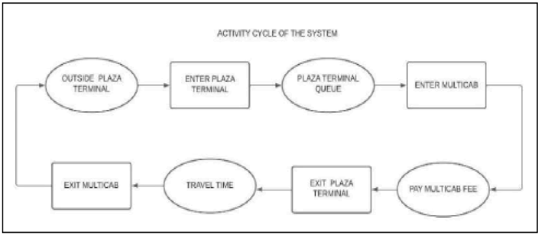
In Figure 1, the flow of the whole plaza terminal is illustrated using the activity cycle. It begins with outside plaza terminal => entering plaza terminal => plaza terminal queue => entering the multicab => pay multicab fee => exit plaza terminal => travel time => exit multicab.
Figure 1: Activity Cycle of the System.
Diagram Flow
Passenger Flow
The passenger flow, shown in Figure 2, starts when passengers enter the plaza terminal and then proceeds through the queue line. After that, when a multicab becomes available and pulled up to the loading station, passengers may enter the multicab and pay for their fee. After a certain amount of time or when the multicab capacity is fully occupied, the multicab will leave the plaza terminal. The next step is for passengers to depart the multicab in between this process or the trip duration. The procedure will then be repeated whereas the passenger is outside the plaza terminal.
Figure 2: Passenger Flow.
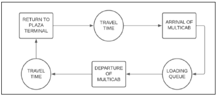
Multicab Flow
The multicab flow process shown in Figure 3 starts when the multicab pulls up to the plaza terminal. Next, there is a loading queue, and if there is a prior multicab there that isn't yet full, the next multicab will wait until the previous multicab is full or reached its certain time limit. There will be a delay from the time it departs and when it arrives back at the plaza terminal to imitate the travel time. Finally, there will be an additional travel period between the arrival of the multicab and its entry into the loading queue.
Figure 3: Multicab Flow
Simulation
Project Timeline
As shown in the Figure 4, the data collection and gathering took two months, starting from April up to May. Researchers have had a tough time gathering and collecting data since most are not available in the eFOI and requesting data were either denied and/or rejected, or until now they haven’t responded. Researchers were able to collect a week's worth of data from the office of the Kapit-Bisig MP and Transport Service Cooperative’s office, an Imus Plaza Terminal, starting from May 22, 2022 to May 28, 2022. For the development of the model, researchers allot a month to work on it and the validation also. For the documentation, as soon as the data were collected, researchers were able to start working on the paper at the end of May up to the month of June 2022.

Figure 4: GANTT chart For Project Timeline.
Input and Output Data Requirements
The Imus Plaza Terminal’s multicab logging dataset was obtained via Imus Plaza’s office with proper legal consent. The paper, as of May 30, 2022, features a timespan of data from the dates May 22, 27, and 28, with the following variables:
• Total number of multicab count.
• Repetitions of travel per each multicab.
• Timestamp record of each travel in and travel out of each multicab, and
• The time difference of waiting spent of each multicab per passenger collection.
These variables represent a proper role in the simulation of the system. The expected output should be the simulated tabular model that contains the number of passengers that rode specific multicabs at a certain given rate.
Starting the Simulation
Both Figure 5 and Figure 6 are the 2D and 3D screenshots of the whole Imus Transport Plaza Terminal designed in Any Logic. The simulation imitates the real life aspect and appearance of the terminal, the multicabs, and the 5 CS363-Modeling-and-Simulation ©2022 road for better and clearer visualization of the actual appearance of the Imus Transport Plaza Terminal.
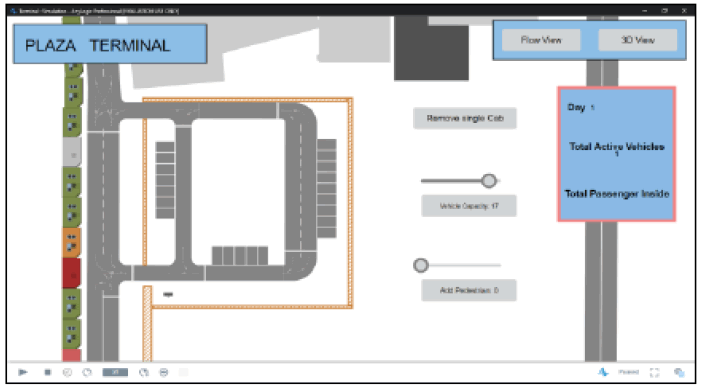
Figure 5: 2D View Model of the Imus Transport Plaza.
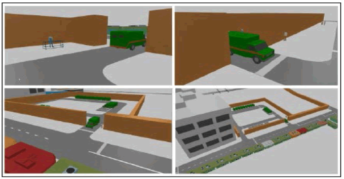
Figure 6: 3D View Model of the Imus Transport Plaza.
Model Flow
The model from Figure 7 is designed to imitate as closely as possible to the real-life event. The model shows the flow of both the multicab and the passenger. The model implemented Poisson distribution in forecasting the number of potential passengers in a certain amount of time and the probable number of available multicab on a particular day.
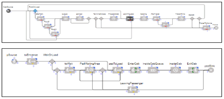
Figure 7: Modeling Flow.
Analysis of the System
Results
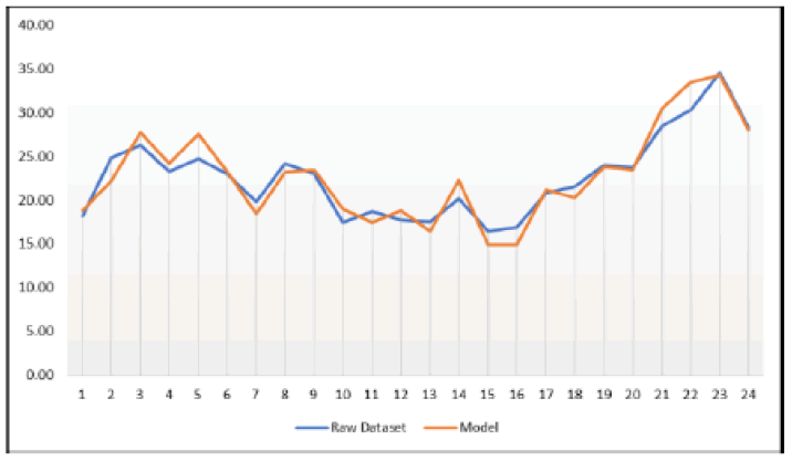
The model produced the number of passengers who departed the terminal. The Graph above shows that the data produced by the model is relative to the raw data that the researchers gathered and collected. The x-axis of the graph represents the number of passengers departed while the y-axis of the graph represents the time of the event which is every 30 minutes.
Graph 1: Data Produced By the Model and Actual Raw Data.
Verification
According to Figure 2 (Passenger Flow), a passenger enters the plaza terminal and waits from a queue line. The passengers will then wait until a multicab arrives (see Figure 3). The arrival of the multicab carries passengers at a set maximum limit, then leaves the terminal and proceeds to their destination. This process repeats in a cyclic routine from 6:19AM (earliest time from the raw dataset) to 7:42PM (latest time from the raw dataset). These processes are evident as shown from the figure below, showcasing the factors written from the raw and unfiltered actual data (Figure 8).
Figure 8:Raw Data From Imus Plaza Terminal.
Validation
Mean Absolute Percentage Error (MAPE) was incorporated into the simulation model that the researchers developed in order to assess the accuracy of the simulated data compared to the real data. The following Table 1 shows the terminal's ridership for every 30 mins from May 22, 2022, through May 28, 2022.
Table 1. The ridership of terminal every day for every 30 mins (actual data).
| Dataset | Sunday | Monday | Tuesday | Wednesday | Thursday | Friday | Saturday | Mean |
|---|---|---|---|---|---|---|---|---|
| 7:00 AM | 20 | 16 | 15 | 10 | 24 | 20 | 22 | 18.14 |
| 7:30 AM | 14 | 32 | 23 | 35 | 15 | 24 | 31 | 24.86 |
| 8:00 AM | 19 | 22 | 32 | 23 | 27 | 33 | 28 | 26.29 |
| 8:30 AM | 24 | 25 | 25 | 35 | 24 | 15 | 17 | 23.29 |
| 9:00 AM | 12 | 19 | 34 | 23 | 33 | 20 | 32 | 24.71 |
| 9:30 AM | 28 | 16 | 33 | 30 | 18 | 20 | 16 | 23.00 |
| 10:00 AM | 15 | 18 | 17 | 18 | 25 | 22 | 23 | 19.35 |
| 10:30 AM | 28 | 22 | 37 | 25 | 22 | 17 | 18 | 24.14 |
| 11:00 AM | 10 | 11 | 31 | 26 | 24 | 32 | 27 | 23.00 |
| 11:30 AM | 25 | 18 | 20 | 15 | 14 | 17 | 13 | 17.45 |
| 12:00 PM | 17 | 14 | 17 | 21 | 29 | 19 | 14 | 18.71 |
| 12:30 PM | 24 | 21 | 29 | 20 | 16 | 8 | 6 | 17.71 |
| 1:00 PM | 13 | 10 | 22 | 25 | 20 | 12 | 21 | 17.57 |
| 1:30 PM | 22 | 31 | 30 | 16 | 11 | 12 | 19 | 20.14 |
| 2:00 PM | 11 | 16 | 9 | 29 | 11 | 15 | 24 | 16.43 |
| 2:30 PM | 16 | 30 | 12 | 9 | 14 | 17 | 18 | 16.96 |
| 1:00 PM | 12 | 13 | 30 | 19 | 12 | 20 | 20 | 20.86 |
| 3:30 PM | 15 | 28 | 16 | 19 | 30 | 21 | 22 | 21.57 |
| 4:00 PM | 18 | 22 | 29 | 25 | 28 | 17 | 29 | 24.00 |
| 4:30 PM | 31 | 33 | 14 | 12 | 27 | 25 | 24 | 23.71 |
| 5:00 PM | 31 | 28 | 24 | 22 | 29 | 30 | 35 | 28.43 |
| 5:30 PM | 16 | 39 | 20 | 45 | 30 | 36 | 26 | 30.25 |
| 6:00 PM | 35 | 35 | 37 | 36 | 33 | 33 | 35 | 34.57 |
| 6:30 PM | 35 | 37 | 20 | 22 | 27 | 33 | 24 | 28.29 |
| Mean | 20.46 | 25.00 | 24.00 | 25.33 | 25.58 | 21.58 | 22.67 |
The researchers will simulate the model to obtain the simulated data that will be compared later after determining the mean on the actual data. As shown in Table 1, the researchers first determined the average number of passengers every 30 minutes during a given time period that would be utilized as a foundation for validating the accuracy of the simulated data. Table 2 contains the data that was obtained by the researchers by simulating the model that uses the Poisson distribution. Thus, the researchers calculated the simulated data's mean and then used the MAPE formula to compare its mean from the actual data to check its accuracy. The result using the MAPE formula in the model is 5.80% for every 30 mins and for daily it has a result of 4.63% (Table 3, 4).
Table 2. Simulated data of the ridership of terminal every day for every 30 mins using mape (output).
|
|
Sunday | Monday | Tuesday | Wednesday | Thursday | Friday | Saturday | Mean | APE |
|---|---|---|---|---|---|---|---|---|---|
| 7:00AM | 21 | 15 | 23 | 20 | 20 | 17 | 16 | 18.86 | 3.94 |
| 7:30 AM | 22 | 21 | 27 | 21 | 25 | 22 | 17 | 22.34 | 10.92 |
| 8.00 AM | 32 | 28 | 21 | 32 | 29 | 20 | 12 | 2771 | 5.43 |
| 8:30 AM | 20 | 21 | 22 | 30 | 26 | 21 | 29 | 24.24 | 3.68 |
| 3:00 AM | 31 | 27 | 10 | 25 | 28 | 25 | 27 | 27.57 | 11.56 |
| 9:30 AM | 32 | 23 | 24 | 17 | 18 | 22 | 26 | 23.29 | 1.24 |
| 10:00 AM | 17 | 14 | 14 | 19 | 19 | 23 | 17 | 18.43 | 7.19 |
| 10:30 AM | 20 | 19 | 13 | 26 | 25 | 21 | 19 | 23.54 | 4.14 |
| 11:00 AM | 18 | 26 | 25 | 21 | 27 | 24 | 23 | 23.41 | 1.86 |
| 11:30 AM | 21 | 15 | 15 | 22 | 19 | 25 | 16 | 2900 | 9.02 |
| 12:00 PM | 18 | 16 | 21 | 18 | 14 | 17 | 18 | 17.45 | 6.87 |
| 13:30 PM | 18 | 14 | 19 | 16 | 27 | 15 | 20 | 1896 | 6.45 |
| 1:00 PM | 20 | 24 | 16 | 0 | 23 | 19 | is | 06.41 | 6.5 |
| 1:50 PM | 21 | 20 | 27 | 55 | 20 | 16 | 17 | 22.29 | 10.64 |
| 2.00 PM | 14 | 17 | 13 | is | 12 | 23 | 10 | 1486 | 9.57 |
| 2:30 PM | 17 | 15 | 18 | 17 | 9 | 10 | 18 | 14.96 | 11.86 |
| 1:00PM | 23 | 24 | 14 | 16 | 17 | 25 | 21 | 21.34 | 1.37 |
| 3:30PM | 15 | 16 | 24 | is | 20 | 23 | 29 | 20.29 | 5.96 |
| 4:00 PM | 21 | 20 | 23 | 20 | 23 | 25 | 27 | 23.86 | 0.6 |
| 4:30PM | 25 | 20 | 21 | 25 | 25 | 20 | so | 23.43 | 1.20 |
| 5:00 PM | 34 | 35 | 11 | so | 32 | 29 | 24 | 50.43 | 7.04 |
| 5:30PM | 34 | 33 | 31 | 30 | 32 | 29 | 35 | 33.41 | 10.38 |
| 6:00PM | 23.46 | 34 | 14 | 33 | 36 | 36 | 23 | 3429 | 0.83 |
| 130PM | 54 | 31 | 24 | 26 | 25 | 25 | 31 | 18.00 | 1.01 |
| Mean | 23.46 | 22.50 | 25.58 | 22.00 | 22.39 | 22.38 | 22.90 | ||
| APE | 14.66 | 2.17 | 1.74 | 5.71 | 3.36 | 3.67 | 1.1 |
Table 3. Result of the simulated model.
| Mape | Result |
|---|---|
| Per 30 min: | 5.8 |
| Daily: | 4.63 |
Table 4. Result of the T test.
| Mape | T-Test |
|---|---|
| Per 30 min: 5.80 | 0.92 |
| Daily: 4.63 | 0.79 |
Scenarios To Be Considered
After producing the model, the researchers were able to simulate the terminal condition when implementing the protocol for covid-19 which limits the capacity of the vehicle as par for the social distancing of the passengers. Using the interface from Figure 5, the researchers were able to change the vehicle's maximum capacity to 50% which only accommodates 8 passengers per vehicle.
By applying the same probability distribution on the acquired dataset but with the constraint of limited passenger capacity per vehicle, the model produced the number of pedestrians shown in Table 5 but the terminal was only able to serve a certain amount of passengers resulting in the loss of potential passengers as shown at Table 6 below:
Table 5. Predicted passenger volume
| Prediction | Sunday | Monday | Tuesday | Wednesday | Thursday | Friday | Saturday |
|---|---|---|---|---|---|---|---|
| 7:00 AM | 14 | 13 | 24 | 19 | 23 | 18 | 15 |
| 7:30 AM | 24 | 30 | 23 | 28 | 27 | 29 | 23 |
| 8:00 AM | 24 | 29 | 19 | 21 | 25 | 25 | 22 |
| 8:30 AM | 26 | 20 | 25 | 20 | 22 | 25 | 22 |
| 9:00 AM | 22 | 28 | 19 | 22 | 18 | 24 | 28 |
| 9:30 AM | 26 | 22 | 27 | 16 | 27 | 22 | 22 |
| 10:00 AM | 21 | 18 | 18 | 20 | 24 | 23 | 22 |
| 10:30 AM | 23 | 30 | 27 | 29 | 20 | 26 | 24 |
| 11:00 AM | 19 | 19 | 13 | 27 | 24 | 19 | 22 |
| 11:30 AM | 20 | 22 | 14 | 22 | 19 | 23 | 15 |
| 12:00 PM | 25 | 18 | 15 | 18 | 16 | 23 | 22 |
| 12:30 PM | 19 | 19 | 16 | 18 | 18 | 13 | 26 |
| 1:00 PM | 12 | 17 | 11 | 17 | 20 | 17 | 20 |
| 1:30 PM | 21 | 12 | 14 | 20 | 15 | 17 | 23 |
| 2:00 PM | 19 | 20 | 22 | 11 | 14 | 21 | 15 |
| 2:30 PM | 19 | 18 | 17 | 15 | 13 | 14 | 17 |
| 3:00 PM | 18 | 20 | 19 | 24 | 18 | 16 | 25 |
| 3:30 PM | 23 | 18 | 15 | 23 | 24 | 26 | 29 |
| 4:00 PM | 19 | 29 | 22 | 29 | 25 | 26 | 26 |
| 4:30 PM | 24 | 23 | 33 | 22 | 28 | 24 | 22 |
| 5:00 PM | 29 | 30 | 33 | 22 | 27 | 23 | 35 |
| 5:30 PM | 30 | 22 | 31 | 32 | 33 | 30 | 33 |
| 6:00 PM | 35 | 33 | 34 | 33 | 34 | 36 | 36 |
| 6:30 PM | 22 | 30 | 26 | 31 | 24 | 29 | 26 |
| TOTAL | 534 | 540 | 517 | 539 | 538 | 559 | 570 |
Table 6. Number of passenger accommodated.
| Serviced Passenger | Sunday | Monday | Tuesday | Wednesday | Thursday | Friday | Saturday |
|---|---|---|---|---|---|---|---|
| 7:00 AM | 14 | 13 | 24 | 19 | 23 | 18 | 15 |
| 7:30 AM | 24 | 30 | 23 | 28 | 27 | 26 | 23 |
| 8:00 AM | 24 | 29 | 19 | 21 | 25 | 28 | 22 |
| 8:30 AM | 26 | 20 | 25 | 20 | 22 | 25 | 22 |
| 9:00 AM | 22 | 28 | 19 | 22 | 18 | 24 | 28 |
| 9:30 AM | 26 | 22 | 27 | 16 | 27 | 22 | 22 |
| 10:00 AM | 21 | 18 | 18 | 20 | 24 | 23 | 22 |
| 10:30 AM | 23 | 30 | 27 | 29 | 20 | 26 | 24 |
| 11:00 AM | 19 | 19 | 13 | 27 | 24 | 19 | 22 |
| 11:30 AM | 20 | 22 | 14 | 22 | 19 | 23 | 15 |
| 12:00 PM | 25 | 18 | 15 | 18 | 16 | 23 | 22 |
| 12:30 PM | 19 | 19 | 16 | 18 | 18 | 13 | 26 |
| 1:00 PM | 12 | 17 | 11 | 17 | 20 | 17 | 20 |
| 1:30 PM | 21 | 12 | 14 | 20 | 15 | 27 | 23 |
| 2:00 PM | 19 | 20 | 22 | 11 | 14 | 21 | 15 |
| 2:30 PM | 19 | 18 | 17 | 15 | 13 | 14 | 17 |
| 3:00 PM | 18 | 20 | 19 | 24 | 18 | 16 | 25 |
| 3:30 PM | 23 | 18 | 15 | 23 | 24 | 26 | 29 |
| 4:00 PM | 19 | 29 | 22 | 25 | 25 | 25 | 26 |
| 4:30 PM | 24 | 23 | 33 | 24 | 28 | 24 | 16 |
| 5:00 PM | 29 | 30 | 33 | 24 | 27 | 23 | 41 |
| 5:30 PM | 30 | 22 | 31 | 24 | 16 | 30 | 32 |
| 6:00 PM | 32 | 26 | 34 | 10 | 36 | 35 | 30 |
| 6:30 PM | 16 | 19 | 26 | 18 | 8 | 24 | 17 |
| Total | 525 | 522 | 517 | 495 | 507 | 554 | 554 |
| Loss | 9 | 18 | 0 | 44 | 31 | 5 | 16 |
Discussion and Conclusion
The simulation of the Imus Plaza Multicab Terminal on its hourly ridership had multiple variables and how to utilize those in order to create a close-to-reality simulation. Using the raw dataset provided by the Imus Plaza Terminal office, the 7 CS363-Modeling-and-Simulation ©2022 usage of Poisson distribution for the cab spawners to provide different curves of probability, and the overall construction of the AnyLogic simulation using the proposed modeling flow, the simulation outputs an average of Mean Absolute Percentage Error (MAPE) of 5.80%; despite of the discrepancies that the aforementioned variables provided. The lesser MAPE conducted between the raw and forecasted data means the simulation is close to what the real world simulation of the ridership in Imus Plaza would be. However, some external variables, for example, the fixed repetition of multicab travels doesn’t reflect that they would immediately return after a successful trip. Instead, in the simulation model at Any Logic, we have set an 80% probability that the vehicle would return again to carry passengers for another trip.
The T-Test (used the internal TTEST function of Microsoft Excel) result shows a p-value of (0.92 for every 30 mins) (0.79 for the daily data) that shows strong significance between the two datasets. The test was run with unequal variance (in relevance for the random seeds and/or probability distributions on the simulation in the Any Logic software). The difference between the two datasets was minimal, expressing how was the real data close in to the simulated model's output data.
Based on the raw dataset and the output of the simulation, the created model is working and properly aligned on the actual data that was obtained at an actual multicab terminal ridership.
References
- Güss, C. D., and. Tuason, M. T. G. "Jeepneys: Values in the streets." Cult. psychol. 14.2 (2008): 211-236.
- Nasution, A. A., Keulana E., and Ladislav B. "Determinant study of conventional transportation and online transportation." Transp. Res. Procedia 44 (2020): 276-282.
- Mateo B., I., et al. "Formalising the jeepney industry in the Philippines–A confirmatory thematic analysis of key transitionary issues." Res. transp. econ 83 (2020): 100839.
- Asaithambi, G., et al. "Study of traffic flow characteristics using different vehicle-following models under mixed traffic conditions." Transp lett. 10.2 (2018): 92-103.
- Kalle, R. K., et al. "Simulation-driven optimization of urban bus transport." WIT Trans Built Environ. 186 (2019): 97-108.
- Hassannayebi, E., et al. "A hybrid simulation model of passenger emergency evacuation under disruption scenarios: A case study of a large transfer railway station." J Simul. 14.3 (2020): 204-228.
- Wibowo, S. S., and Siti R. F. "Queuing analysis using Viswalk for check-in counter: Case study of Lombok Praya International Airport." MATEC Web of Conferences. Vol. 181. EDP Sciences, 2018.
- Alexandre G. D. B., and David D. T. "Quantitative analysis of passenger and baggage security screening at airports." J Adv Transp. 41.2 (2007): 171-193.
- Munasingha, K., and Varuna A. "Discrete event simulation method to model passenger processing at an international airport." 2020 Moratuwa Eng Res Conf (MERCon), IEEE, 2020.
- Ghosh, J. K., et al. An introduction to Bayesian analysis: theory and methods. Vol. 725. New York: Springer, 2006.
[Google Scholar] [Cross Ref]
- Inouye, D. I., et al. "A review of multivariate distributions for count data derived from the Poisson distribution." Wiley Interdiscip. Rev: Comput Stat. 9.3 (2017): e1398.
- Sharma, D. K., et al. "An Efficient Python Approach for Simulation of Poisson Distribution." 2021 7th Int Conf Adv Comput Commun Syst (ICACCS). Vol. 1. IEEE, 2021.
